Daten Typen & Vektoren & For Loops

rstatsZH - Data Science mitR

Lars Schöbitz

Oct 28, 2025

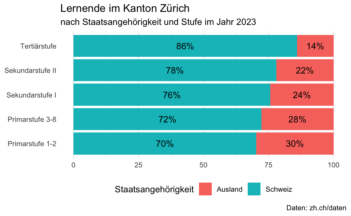
# Die Daten werden hier direkt von der URL gelesen. Bei einem Update der Daten
# wird hier immer auf die aktuellste Version zugegriffen.
link <- "https://www.web.statistik.zh.ch/ogd/data/bista/ZH_Uebersicht_alle_Lernende.csv"

# Hier wird nun das Objekt "link" genutzt um die CSV zu lesen
lernende_in <- read_csv(file = link)

Rows: 2972 Columns: 10
── Column specification ────────────────────────────────────────────────────────
Delimiter: ","
chr  (7): Kanton, Stufe, Schultyp, Geschlecht, Staatsangehoerigkeit, Traeger...
dbl  (2): Jahr, Anzahl
date (1): Stand

ℹ Use `spec()` to retrieve the full column specification for this data.
ℹ Specify the column types or set `show_col_types = FALSE` to quiet this message.

lernende <- lernende_in |> 
    filter(Geschlecht != 2) |> 
    mutate(Geschlecht = case_when(
        Geschlecht %in% c("m", "M") ~ "männlich",
        Geschlecht %in% c("f", "F") ~ "weiblich"
    )) |> 
    mutate(Traegerschaft = case_when(
        Traegerschaft == "oef" ~ "öffentlich",
        Traegerschaft == "priv" ~ "privat"
    )) |>
    mutate(Finanzierung = case_when(
        Finanzierung == "oef" ~ "öffentlich",
        Finanzierung == "priv" ~ "privat"))

lernende_max <- lernende |> 
    filter(Jahr == max(Jahr))

lernende_max_stufe_staat_sum <- lernende_max |> 
    group_by(Stufe, Staatsangehoerigkeit)  |> 
    summarise(
        Total = sum(Anzahl)
    ) |> 
    mutate(Prozent = Total / sum(Total) * 100)

`summarise()` has grouped output by 'Stufe'. You can override using the
`.groups` argument.

Modul 5 - Zusatzaufgabe 3

ggplot(data = lernende_max_stufe_staat_sum,
       mapping = aes(x = Stufe, 
                     y = Prozent, 
                     fill = Staatsangehoerigkeit)) +
    coord_flip() +
    geom_col() +
    geom_text(aes(label = paste0(round(Prozent, 0), "%")),  
              position = position_stack(vjust = 0.5)) +
    labs(title = "Lernende im Kanton Zürich ",
         subtitle = "nach Staatsangehörigkeit und Stufe im Jahr 2023",
         fill = "Staatsangehörigkeit",
         caption = "Daten: zh.ch/daten",
         y = NULL,
         x = NULL) +
    theme_minimal() +
    theme(legend.position = "bottom", 
          panel.grid.major.y = element_blank())

Lernziele (für diese Woche)

lernziele <- readr::read_csv(here::here("data/tbl-01-rstatszh-lernziele.csv")) |> 
  dplyr::filter(modul == params$modul) |>
  dplyr::pull(lernziele)

Rows: 36 Columns: 4
── Column specification ────────────────────────────────────────────────────────
Delimiter: ","
chr  (2): titel, lernziele
dbl  (1): modul
dttm (1): datum

ℹ Use `spec()` to retrieve the full column specification for this data.
ℹ Specify the column types or set `show_col_types = FALSE` to quiet this message.

Die Lernenden können die Bedeutung von Vektoren mit Bezug auf einen Dataframe erläutern.
Die Lernenden können drei verschiedene Methoden anwenden um auf einen Vektor in einem dataframe zuzugreifen.
Die Lernenden können die vier wichtigsten atomaren Vektortypen in R auflisten.
Die Lernenden können einen for loop verwenden, um durch die Elemente eines Vektors in einem Dataframe zu iterieren und spezifische Operationen auf jedes Element anzuwenden.

library(tidyverse)
library(knitr)
library(gt)
library(epoxy)
library(palmerpenguins)


Attaching package: 'palmerpenguins'

The following objects are masked from 'package:datasets':

    penguins, penguins_raw

library(countdown)

ggplot2::theme_set(ggplot2::theme_gray(base_size = 16))

waste_data_lord1 <- read_csv("https://raw.githubusercontent.com/rbtl-fs22/rbtl-fs22-data/main/raw_data/lord-of-the-bins/04-05-2022_rbtl_data_sheet1.csv")

Rows: 5 Columns: 12
── Column specification ────────────────────────────────────────────────────────
Delimiter: ","
chr  (2): location, day_of_collection
dbl (10): objid, bin_id, bin_id_2, non_recyclables_ Kg, pet_Kg, metal_conten...

ℹ Use `spec()` to retrieve the full column specification for this data.
ℹ Specify the column types or set `show_col_types = FALSE` to quiet this message.

waste_data_lord2 <- read_csv("https://raw.githubusercontent.com/rbtl-fs22/rbtl-fs22-data/main/raw_data/lord-of-the-bins/04-05-2022_rbtl_data_sheet2.csv")

Rows: 5 Columns: 12
── Column specification ────────────────────────────────────────────────────────
Delimiter: ","
chr  (2): location, day_of_collection
dbl (10): objid, bin_id, bin_id_2, non_recyclables_ Kg, pet_Kg, metal_conten...

ℹ Use `spec()` to retrieve the full column specification for this data.
ℹ Specify the column types or set `show_col_types = FALSE` to quiet this message.

survey_data <- read_csv("https://raw.githubusercontent.com/rbtl-fs22/rbtl-fs22-data/main/raw_data/partners-in-grime/2022-05-04_survey-data.csv") |> 
  mutate(id = seq(1:n()))

Rows: 22 Columns: 15
── Column specification ────────────────────────────────────────────────────────
Delimiter: ","
chr (14): Date Started, age, job, residence_situation, residence_type, locat...
dbl  (1): residence_distance

ℹ Use `spec()` to retrieve the full column specification for this data.
ℹ Specify the column types or set `show_col_types = FALSE` to quiet this message.

survey_data_small <- survey_data |> 
  select(id, job, price_glass)

survey_data_tidy <- survey_data |> 
  select(id, job, residence_situation, starts_with("price")) |> 
  pivot_longer(cols = starts_with("price"),
               names_to = "waste_category",
               values_to = "price") |> 
  mutate(waste_category = str_remove(waste_category, pattern = "price_")) |> 
  mutate(price_new = case_when(
    price == "5 to 10" ~ "7.5",
    price == "05-Oct" ~ "7.5",
    str_detect(price, pattern = "20") == TRUE ~ "20",
    str_detect(price, pattern = "See comment") == TRUE ~ NA_character_,
    TRUE ~ price
  )) |> 
  mutate(price = as.numeric(price_new)) |> 
  select(-price_new)

Warning: There was 1 warning in `mutate()`.
ℹ In argument: `price = as.numeric(price_new)`.
Caused by warning:
! NAs introduced by coercion

#survey_data_tidy |>
#  count(job, residence_situation, waste_category, price) |>
#  ggplot(aes(x = factor(price), y = n, fill = job)) +
#  geom_col()
#

waste_data <- bind_rows(waste_data_lord1, waste_data_lord2)

waste_data_untidy <- waste_data |> 
  filter(!is.na(objid)) |> 
  rename(non_recyclable_Kg = `non_recyclables_ Kg`,
         recyclable_Kg = recyclables_Kg) |>
  relocate(c(recyclable_Kg, non_recyclable_Kg), .before = weight_total_kg) |> 
  select(objid, location, pet_Kg:weight_total_kg) |> 
  mutate(objid = factor(objid)) |>
  rename_with(~str_remove(.x, "_Kg|_kg")) |> 
  rename_with(~str_remove(.x, "_content")) |> 
  rename(total = weight_total)


waste_category_levels <- c("glass", "metal_alu", "paper", "pet", "other")

waste_data_tidy <- waste_data_untidy |> 
  select(objid:paper, non_recyclable) |> 
  rename(other = non_recyclable) |> 
  mutate(objid = factor(objid)) |>
  pivot_longer(cols = pet:other,
               names_to = "waste_category",
               values_to = "weight") |> 
  mutate(waste_category = factor(waste_category, levels = waste_category_levels)) |> 
  mutate(type = case_when(
    waste_category == "other" ~ "non_recyclable",
    TRUE ~ "recyclable")) |> 
  relocate(type, .before = weight) |> 
  group_by(objid) |> 
  mutate(percent = weight / sum(weight) * 100)

waste_data_tidy |> 
  write_rds(here::here("folien/daten/processed/waste-characterisation-lord-of-the-bins-tidy.rds"))

waste_data_tidy |> 
  group_by(location, waste_category) |> 
  summarise(weight = mean(weight)) |> 
  group_by(location) |> 
  mutate(percent = weight / sum(weight) * 100) 

waste_data_tidy |> 
  
  ggplot(mapping = aes(x = waste_category, y = weight, color = type)) +
  geom_boxplot() +
  geom_jitter(width = 0.2) +
  facet_wrap(~location)

waste_data_tidy |> 
  ggplot(mapping = aes(x = objid, y = weight)) +
  geom_col() 

waste_data_tidy |> 
  ggplot(mapping = aes(x = objid, y = weight, fill = waste_category)) +
  geom_col() 

waste_data_tidy |> 
  ggplot(mapping = aes(x = waste_category, y = percent, color = type)) +
  geom_boxplot() +
  geom_jitter(width = 0.2) +
  facet_wrap(~location)


waste_data_tidy |> 
  ggplot(aes(x = objid, y = percent, fill = waste_category)) +
  geom_col() 

waste_data_tidy |> 
  ggplot(aes(x = objid, y = percent, fill = type)) +
  geom_col() 

waste_data_tidy |> 
  ggplot(aes(x = objid, y = percent, fill = location)) +
  geom_col() +
  facet_wrap(~waste_category, ncol = 5)

Daten Typen und Vektoren

Warum sind Daten Typen wichtig?

via GIPHY

Beispiel: Recycling Umfrage in Zürich

Eine Umfrage zum Recycling-Verhalten in der Stadt Zürich:

job: Was ist dein Beruf?
price_glass: Welchen monatlichen Betrag wärst du bereit für eine Metall/Glas-Tonne vor deinem Haus zu zahlen?

id	job	price_glass
1	Student	0
2	Retired	0
3	Other	0
4	Employed	10
5	Employed	See comment
6	Student	5-10
7	Student	0
8	Retired	0
9	Student	10
10	Employed	0
11	Employed	20 (2chf per person with 10 people in the WG)
12	Student	10
13	Student	10
14	Employed	0
15	Student	10
16	Student	0
17	Employed	5-10
18	Other	0
19	Student	0
20	Employed	10
21	Employed	0
22	Employed	5

Oh warum klappt das nicht?!

survey_data_small |> 
  summarise(mean_price_glass = mean(price_glass))

Warning: There was 1 warning in `summarise()`.
ℹ In argument: `mean_price_glass = mean(price_glass)`.
Caused by warning in `mean.default()`:
! argument is not numeric or logical: returning NA

# A tibble: 1 × 1
  mean_price_glass
             <dbl>
1               NA

Oh warum klappt das immernoch nicht!!??

survey_data_small |> 
  summarise(mean_price_glass = mean(price_glass, na.rm = TRUE))

Warning: There was 1 warning in `summarise()`.
ℹ In argument: `mean_price_glass = mean(price_glass, na.rm = TRUE)`.
Caused by warning in `mean.default()`:
! argument is not numeric or logical: returning NA

# A tibble: 1 × 1
  mean_price_glass
             <dbl>
1               NA

Atme tief durch und schau dir deine Daten an

id	job	price_glass
1	Student	0
2	Retired	0
3	Other	0
4	Employed	10
5	Employed	See comment
6	Student	5-10
7	Student	0
8	Retired	0
9	Student	10
10	Employed	0
11	Employed	20 (2chf per person with 10 people in the WG)
12	Student	10
13	Student	10
14	Employed	0
15	Student	10
16	Student	0
17	Employed	5-10
18	Other	0
19	Student	0
20	Employed	10
21	Employed	0
22	Employed	5

Atme tief durch und schau dir deine Daten an

# A tibble: 22 × 3
      id job      price_glass
   <int> <chr>    <chr>      
 1     1 Student  0          
 2     2 Retired  0          
 3     3 Other    0          
 4     4 Employed 10         
 5     5 Employed See comment
 6     6 Student  5-10       
 7     7 Student  0          
 8     8 Retired  0          
 9     9 Student  10         
10    10 Employed 0          
# ℹ 12 more rows

Ein sehr typischer Schritt in der Datenbereinigung!

survey_data_small |> 
  mutate(price_glass_new = case_when(
    price_glass == "5-10" ~ "7.5",
    price_glass == "05-Oct" ~ "7.5",
    str_detect(price_glass, pattern = "2chf") == TRUE ~ "2",
    str_detect(price_glass, pattern = "See comment") == TRUE ~ NA_character_,
    TRUE ~ price_glass
  ))

Ein sehr typischer Schritt in der Datenbereinigung!

id	job	price_glass_new	price_glass
1	Student	0	0
2	Retired	0	0
3	Other	0	0
4	Employed	10	10
5	Employed	NA	See comment
6	Student	7.5	5-10
7	Student	0	0
8	Retired	0	0
9	Student	10	10
10	Employed	0	0
11	Employed	2	20 (2chf per person with 10 people in the WG)
12	Student	10	10
13	Student	10	10
14	Employed	0	0
15	Student	10	10
16	Student	0	0
17	Employed	7.5	5-10
18	Other	0	0
19	Student	0	0
20	Employed	10	10
21	Employed	0	0
22	Employed	5	5

Summarise? Argh!!!!

survey_data_small |> 
  mutate(price_glass_new = case_when(
    price_glass == "5-10" ~ "7.5",
    price_glass == "05-Oct" ~ "7.5",
    str_detect(price_glass, pattern = "2chf") == TRUE ~ "2",
    str_detect(price_glass, pattern = "See comment") == TRUE ~ NA_character_,
    TRUE ~ price_glass
  )) |> 
  summarise(mean_price_glass = mean(price_glass_new, na.rm = TRUE))

Warning: There was 1 warning in `summarise()`.
ℹ In argument: `mean_price_glass = mean(price_glass_new, na.rm = TRUE)`.
Caused by warning in `mean.default()`:
! argument is not numeric or logical: returning NA

# A tibble: 1 × 1
  mean_price_glass
             <dbl>
1               NA

Respektiere deine Daten Typen!

Den Durchschnitt von einem Vektor mit Typ “character” zu berechnen ist nicht möglich.

survey_data_small |> 
  mutate(price_glass_new = case_when(
    price_glass == "5-10" ~ "7.5",
    price_glass == "05-Oct" ~ "7.5",
    str_detect(price_glass, pattern = "2chf") == TRUE ~ "2",
    str_detect(price_glass, pattern = "See comment") == TRUE ~ NA_character_,
    TRUE ~ price_glass
  ))

# A tibble: 22 × 4
      id job      price_glass price_glass_new
   <int> <chr>    <chr>       <chr>          
 1     1 Student  0           0              
 2     2 Retired  0           0              
 3     3 Other    0           0              
 4     4 Employed 10          10             
 5     5 Employed See comment <NA>           
 6     6 Student  5-10        7.5            
 7     7 Student  0           0              
 8     8 Retired  0           0              
 9     9 Student  10          10             
10    10 Employed 0           0              
# ℹ 12 more rows

Respektiere deine Daten Typen!

survey_data_small |> 
  mutate(price_glass_new = case_when(
    price_glass == "5-10" ~ "7.5",
    price_glass == "05-Oct" ~ "7.5",
    str_detect(price_glass, pattern = "2chf") == TRUE ~ "2",
    str_detect(price_glass, pattern = "See comment") == TRUE ~ NA_character_,
    TRUE ~ price_glass
  )) |> 
  mutate(price_glass_new = as.numeric(price_glass_new)) |> 
  summarise(mean_price_glass = mean(price_glass_new, na.rm = TRUE))

# A tibble: 1 × 1
  mean_price_glass
             <dbl>
1             3.90

Ich bin dran: Vektoren und Iteration mit for-Schleifen

Zurücklehnen und Fragen stellen!

countdown(minutes = 40)

40:00

Pause machen

Bitte steh auf und beweg dich.

countdown(minutes = 10)

10:00

Ihr seid dran: `02-iteration-ihr.qmd`

Öffne posit.cloud in deinem Browser (verwende dein Lesezeichen).
Öffne den rstatszh-k011 Arbeitsbereich (Workspace) für den Kurs.
Klicke auf Start neben md-06-uebungen.
Suche im Dateimanager im Fenster unten rechts die Datei 02-iteration-ihr.qmd und klicke darauf, um sie im Fenster oben links zu öffnen.
Folge den Anweisungen in der Datei.

countdown(40)

40:00

Zeitpuffer: Modul 6 Uebungen

Kann ich noch etwas zu den Übungen in 02-iteration-ihr.qmd sagen?

countdown(5)

05:00

Pause machen

Bitte steh auf und beweg dich.

countdown(minutes = 5)

05:00

Sensitive Daten und GitHub

schützenswerte Daten dürfen nicht auf GitHub

schützenswerte Daten:

verletzen die Privatsphäre (z.B. Einzeldaten)
sind sicherheitskritisch (z.B. Passwörter)
unterliegen Drittrechten (z.B. Copyrights)

Lösung: `.gitignore`

Dateien und Verzeichnisse in .gitignore eintragen
werden nicht auf GitHub hochgeladen

Daten teilen

Damit eine Analyse reproduzierbar ist, müssen die Daten für andere zugänglich sein. Die Dateien können auf anderen Wegen geteilt werden, z.B. per E-Mail, USB-Stick, Cloud-Dienst, etc.

Informationssicherheit

Folgender Dateipfad enthält Informationen zum Dateisystem und sollte nicht auf GitHub hochgeladen werden:

read_csv("C:/Users/Lars/Documents/projekt-umfrage/daten/umfrage_daten.csv")

Ein guter Weg dies zu vermeiden ist die Verwendung von relativen Pfaden in Kombination mit der here() Funktion aus dem gleichnamigen R-Paket here. Im RStudio Project / GitHub Repository mit dem Namen projekt-umfrage:

read_csv(here::here("daten/umfrage_daten.csv"))

Wir sind dran: `03-gitignore-wir.qmd` & `docs/04-dateipfade.qmd`

Öffne posit.cloud in deinem Browser (verwende dein Lesezeichen).
Öffne den rstatszh-k011 Arbeitsbereich (Workspace) für den Kurs.
Klicke auf Continue neben md-06-uebungen.
Suche im Dateimanager im Fenster unten rechts die Datei 03-gitignore-wir.qmd und klicke darauf, um sie im Fenster oben links zu öffnen.

countdown(20)

20:00

Zeitpuffer: Modul 6 Uebungen

Kann ich noch etwas zum heutigen Modul erklären?

countdown(10)

10:00

Zusatzaufgaben Modul 6

Modul 6 Dokumentation

rstatszh-k011.github.io/website//module/md-06.html

Zusatzaufgaben Abgabedatum

Abgabedatum: Dienstag, 04. November

Danke

Danke! 🌻

Folien erstellt mit revealjs und Quarto: https://quarto.org/docs/presentations/revealjs/

Access slides als PDF auf GitHub

Alle Materialien sind lizenziert unter Creative Commons Attribution Share Alike 4.0 International.

Daten Typen & Vektoren & For Loops

Modul 5 - Zusatzaufgabe 3

Lernziele (für diese Woche)

Daten Typen und Vektoren

Warum sind Daten Typen wichtig?

Beispiel: Recycling Umfrage in Zürich

Oh warum klappt das nicht?!

Oh warum klappt das immernoch nicht!!??

Atme tief durch und schau dir deine Daten an

Atme tief durch und schau dir deine Daten an

Ein sehr typischer Schritt in der Datenbereinigung!

Ein sehr typischer Schritt in der Datenbereinigung!

Summarise? Argh!!!!

Respektiere deine Daten Typen!

Respektiere deine Daten Typen!

Ich bin dran: Vektoren und Iteration mit for-Schleifen

Pause machen

Ihr seid dran: 02-iteration-ihr.qmd

Zeitpuffer: Modul 6 Uebungen

Pause machen

Sensitive Daten und GitHub

schützenswerte Daten dürfen nicht auf GitHub

Lösung: .gitignore

Informationssicherheit

Wir sind dran: 03-gitignore-wir.qmd & docs/04-dateipfade.qmd

Zeitpuffer: Modul 6 Uebungen

Zusatzaufgaben Modul 6

Modul 6 Dokumentation

Zusatzaufgaben Abgabedatum

Danke

Danke! 🌻

Ihr seid dran: `02-iteration-ihr.qmd`

Lösung: `.gitignore`

Wir sind dran: `03-gitignore-wir.qmd` & `docs/04-dateipfade.qmd`